← Back to index

2D phonons dispersion

Authors: Stéphane Nilsson and Giovanni Pizzi

Original notebook: Phonon_2D.ipynb

This notebook extends the notion of phonons to the 2D case. In this notebook, the link between the reciprocal space and the band dispersion plot along certain path is made explicit. The wave can now be transversal as opposed to longitudinal only in the 1D phonon case. A simple example, the square lattice, and a more complex one, the honeycomb lattice, are presented.

Goals

• Explore the available phonons in 2D for different lattices.
• Understand how the dispersion plots are constructed along a path.
• Discover the importance of highly symmetrical points.

Background theory

More on the background theory.

Tasks and exercises

1. Is the honeycomb lattice a 2D Bravais lattice?

   Solution

   The honeycomb lattice is not a 2D Bravais lattice. If you look at the surroundings of two nearest-neighbours atoms, they will differ. The honeycomb lattice is an hexagonal lattice with a two atoms basis. This two atoms basis explains the appearance of an acoustic and optical modes in the phonon dispersion.

2. What are the direct and reciprocal space vectors of the square lattice and honeycomb lattice?

   Solution

   In 2D, the reciprocal space vectors can be obtained from the following formula :

   $$\begin{pmatrix} b_{1x}&b_{1y}\\ b_{2x}&b_{2y} \end{pmatrix}=\frac{2\pi}{a_{1x}a_{2y}-a_{1y}a_{2x}}\begin{pmatrix} a_{2y}&-a_{2x}\\ -a_{1y}&a_{1x} \end{pmatrix}$$

   which solves the reciprocal lattice condition $b_i\cdot a_j=2\pi\delta_{ij}$.

   The square lattice basis vectors are $a_1=a\begin{bmatrix}1\\0 \end{bmatrix}$, $a_2=a\begin{bmatrix}0\\1 \end{bmatrix}$

   The honeycomb lattice basis vectors are $a_1=a\begin{bmatrix}\frac{3}{2}\\ \frac{\sqrt{3}}{2} \end{bmatrix}$, $a_2=a\begin{bmatrix}\frac{3}{2}\\ \frac{-\sqrt{3}}{2} \end{bmatrix}$, with $a$ the nearest neighbour distance.

   The reciprocal vectors are thus :

   • Square lattice : $b_1=\frac{2\pi}{a}\begin{bmatrix}1\\0 \end{bmatrix}$ and $b_2=\frac{2\pi}{a}\begin{bmatrix}0\\1 \end{bmatrix}$
   • Honeycomb lattice : $b_1=\frac{2\pi}{a}\begin{bmatrix}\frac{1}{3}\\ \frac{1}{\sqrt{3}} \end{bmatrix}$ and $b_2=\frac{2\pi}{a}\begin{bmatrix}\frac{1}{3}\\ -\frac{1}{\sqrt{3}} \end{bmatrix}$

3. How many nearest neighbours does the square lattice have? For the honeycomb lattice? How many next-nearest neighbours? Give the coordinate of the nearest and next-nearest neighbours.

   Solution

   The square lattice has 4 nearest neighbours and 4 next-nearest ones. The honeycomb lattice has 3 nearest neighbours and 6 next-nearest ones.

   The positions are :

   • Square lattice : 1st neighbours :$a\begin{bmatrix}1\\0 \end{bmatrix}$, $a\begin{bmatrix}-1\\0 \end{bmatrix}$, $a\begin{bmatrix}0\\1 \end{bmatrix}$, $a\begin{bmatrix}0\\-1 \end{bmatrix}$, 2nd neighbours : $a\begin{bmatrix}1\\1 \end{bmatrix}$, $a\begin{bmatrix}-1\\1 \end{bmatrix}$, $a\begin{bmatrix}1\\-1 \end{bmatrix}$, $a\begin{bmatrix}-1\\-1 \end{bmatrix}$
   • Honeycomb lattice : 1st neighbours : $a\begin{bmatrix}-1\\0 \end{bmatrix}$, $a\begin{bmatrix}\frac{1}{2}\\ \frac{\sqrt3}{2} \end{bmatrix}$, $a\begin{bmatrix}\frac{1}{2}\\ -\frac{\sqrt3}{2} \end{bmatrix}$, 2nd neighbours : $a\begin{bmatrix}\frac{3}{2}\\ \frac{\sqrt3}{2} \end{bmatrix}$, $a\begin{bmatrix}\frac{1}{2}\\ -\frac{\sqrt3}{2} \end{bmatrix}$, $a\begin{bmatrix}-\frac{1}{2}\\ \frac{\sqrt3}{2} \end{bmatrix}$, $a\begin{bmatrix}-\frac{1}{2}\\ -\frac{\sqrt3}{2} \end{bmatrix}$, $a\begin{bmatrix}0\\ \sqrt3 \end{bmatrix}$, $a\begin{bmatrix}0\\ -\sqrt3 \end{bmatrix}$

   (N.B. The signs may vary depending which atom you selected.)

4. Where are the high symmetry point located in the square lattice? And for the honeycomb one? What particularity do you observe at those points?

   Solution

   The high symmetry points are found at the corners and center of edges of the first BZ. The positions are :

   • Square lattice : $\mathbf{M}=\frac{2\pi}{a}\begin{bmatrix}1\\1 \end{bmatrix}$, $\mathbf{X}=\frac{2\pi}{a}\begin{bmatrix}1\\0 \end{bmatrix}$
   • Honeycomb lattice : $\mathbf{K}=\frac{2\pi}{a}\begin{bmatrix}\frac{1}{3} \\\frac{1}{3\sqrt{3}} \end{bmatrix}$, $\mathbf{M}=\frac{2\pi}{a}\begin{bmatrix}\frac{1}{3} \\0 \end{bmatrix}$

   At the high symmetry points, the phonon will also show high symmetries. This can be seen from atoms moving completely out-of-phase or in-phase.

5. How would you compute the dispersion curve along a path? Take the $\Gamma-\mathbf{M}$ path of the square lattice.

   Solution

   Given a dispersion relation $w(k)$, the frequency $w$ is computed for $n$ $k$ points evenly spaced in between two points. In the case of the $\Gamma-\mathbf{M}$ path, the $k$ points are taken along the line $\lambda=\Gamma+(\mathbf{M}-\Gamma)$ which results in points of the form $k=c\begin{bmatrix}1 \\1 \end{bmatrix}$ where $c\in[0,1]$.

6. Look at the square lattice $\mathbf{X}$ point. What is the difference between longitudinal and transverse waves?

   Solution

   In longitudinal waves the atoms displacement is parallel to the wave propagation direction, whereas in transverse waves the atoms displacement is perpendicular to the wave propagation direction. An example of longitudinal wave are sound waves. Instead, waves on the water surface are transversal.

Interactive visualization

Latticesquarehoneycomb

Phononlongitudinaltransverse

C₁2.0C₂1.0

Click on the plots to get the corresponding phonon

PauseCamera axis:xyzLeft drag: rotate · wheel: zoom · right drag: translate

Loading 3D view…

Animation speed1.0Arrow amplitude2.0Oscillation amplitude0.06Atom radius0.10Arrow radius0.05Show arrows

Repetitions:x:y:

Using the interactive visualization

Phonon viewer

The bottom view shows an interactive animation of a lattice vibration.

• Use the Play / Pause button to start and stop the animation (it also stops while the view is off-screen).

• Rotate the surface by left clicking and dragging.

• Translate the surface by right clicking and dragging.

You can reset the view by clicking the corresponding ‘camera axis’ buttons.

Controls

Above the view are two plots.

The plot on the left shows the first Brillouin zone of either a square or honeycomb lattice. The plot on the right shows the dispersion relation along a specific path.

Click on either plot to get the corresponding lattice vibration.

The type of phonon, acoustic, optical, transverse or longitudinal, can be selected by ticking the corresponding box.

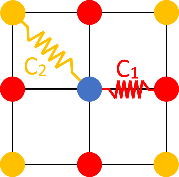
The elastic constant between 1st, 2nd and 3rd nearest neighboors can be varying by sliding the $C_1, C_2$ and $C_3$ sliders.

Appearance

Under the view are parameters related to showing arrows along the oscillations or modifying the atoms appearance.