← Go back to the interactive notebook

Background theory: Introduction to phonons

Original notebook: theory_phonon_1d.ipynb


Introduction

Phonons are a quantum mechanical description of elemental vibrations in the solid. Like photons are quantized light waves, phonons can be thought of quantized sound waves. Arising from the elastic arrangement of atoms, phonons play an important role in the study of thermal and electrical properties of materials. They describe the vibrational motion of a lattice of atoms oscillating at a single frequency, analogous to normal modes in classical mechanics. Any lattice vibrations can then be described as a superposition of those normal modes.

1D monoatomic chain

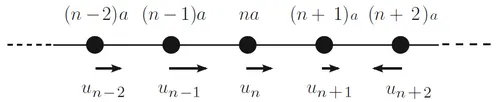
Let’s now consider the case of a 1D monoatomic chain in which only the first neighbours interactions are considered. Let Rn=naR_n=na be the position of atom nn, Rn+1=(n+1)aR_{n+1}=(n+1)a the position of atom n+1n+1, etc., as shown in Fig. 1. The classical equation of motion of the nn-th atom of mass MM in position Rn+un(t)R_n+u_n(t) under the force FnF_n is:

Mu¨n=−C1(un−1−un)−C1(un+1−un)=−C1(2un−un−1−un+1)(1)M\ddot u_n = -C_1(u_{n-1}-u_{n})-C_1(u_{n+1}-u_n)=-C_1(2u_n-u_{n-1}-u_{n+1}) \qquad (1)

where n−1n-1 and n+1n+1 are the two neighbouring atoms and C1C_1 the force constant between neighbours.

Solutions of the differential equation are in the form of traveling wave, periodic in space and time, of the type :

un(t)=Aei(k⋅Rn−ωt)(2)u_n(t)=Ae^{i(k\cdot R_n-\omega t)} \qquad (2)

where AA is the amplitude of the displacement, kk is the phonon wave vector and ω\omega its frequency.

Plugging Eq.2 into Eq.1 results in

−Mω2eikne−iωt=−C1(2eikne−iωt−eikne−iωte−ika−eikne−iωteika)Mω2=−C1(2−e−ika−eika)(3)\begin{aligned} -M \omega^2 \cancel{e^{ikn}}\cancel{e^{-i\omega t}} & =-C_1(2\cancel{e^{ikn}}\cancel{e^{-i\omega t}}-\cancel{e^{ikn}}\cancel{e^{-i\omega t}}e^{-ika}-\cancel{e^{ikn}}\cancel{e^{-i\omega t}}e^{ika}) \\ M \omega^2 & =-C_1(2-e^{-ika}-e^{ika}) \qquad (3) \end{aligned}

Eq.3 gives us a direct relation between ω\omega and kk, which is called the dispersion relation.

Schematic of the 1D monoatomic chain
Figure 1: Schematic of the 1D monoatomic chain.

1D diatomic chain

Let us now consider the case in which two atoms site in the unit cell, with mass M1M_1 and M2M_2. The positions are given by Rn(1)=naR_n^{(1)}=na and Rn(2)=na+12aR_n^{(2)}=na+\frac{1}{2}a. uu is the displacement of atom 1 and vv is the displacement of atom 2. The system of equations is then
M1u¨n=−C1(2un−vn−1−vn+1)(4)M2v¨n=−C1(2vn−un−1−un+1)(5)\begin{aligned} M_1\ddot u_n & =-C_1(2u_n-v_{n-1}-v_{n+1}) \qquad (4) \\ M_2\ddot v_n & =-C_1(2v_n-u_{n-1}-u_{n+1}) \qquad (5) \end{aligned}

The solution of such a system is given by

un(t)=A1ei(k⋅Rn(1)−ωt)andvn(t)=A2ei(k⋅Rn(2)−ωt)(6)u_n(t)=A_1e^{i(k\cdot R_n^{(1)}-\omega t)}\qquad \text{and}\qquad v_n(t)=A_2e^{i(k\cdot R_n^{(2)}-\omega t)} \qquad(6)

Inserting Eq.6 into Eq.4 and Eq.5 gives :

−M1ω2A1=−C(2A1−A2e−ika/2−A2eika/2)−M2ω2A2=−C(2A2−A1e−ika/2−A1eika/2)\begin{aligned} & -M_{1} \omega^{2} A_{1}=-C\left(2 A_{1}-A_{2} e^{-i k a / 2}-A_{2} e^{i k a / 2}\right) \\ & -M_{2} \omega^{2} A_{2}=-C\left(2 A_{2}-A_{1} e^{-i k a / 2}-A_{1} e^{i k a / 2}\right) \end{aligned}

which is equal to solving the eigenvalue problem :

CA⃗=ω2A⃗\mathbf{C}\vec{A}=\omega^2 \vec{A}

where Aω⃗=[A1A2]\vec{A_\omega}=\begin{bmatrix}A_1\\A_2\end{bmatrix}. Aω⃗\vec{A_\omega} is the eigenvector corresponding to the eigenvalue ω\omega.

Further references

G. Grosso and G. Pastori Parravicini, Solid state physics, Second edition. Amsterdam: Academic Press, an imprint of Elsevier, 2014.