← Go back to the interactive notebook
Background Theory: Numerical Solution of the Schrödinger Equation for the Double Square Well Potential
Original notebook: theory_2quantumwells.ipynb
Introduction
We implemented a numerical method to solve the Schrödinger equation for the one-dimensional double square well potential in this notebook. The numerical method and its algorithm are explicitly outlined in the “Numerical Solution of the Schrödinger Equation for a One Dimensional Quantum Well” notebook.
DSWP model for H molecule
The double square well potential model is a simple but efficient way to describe real molecular or material systems. For instance, the DSWP model can be used to describe the H molecule.
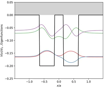
In the H molecule, there are two identical protons and two electrons. We can simplify the potential as two identical square well potential as shown in the figure above. The two lowest energy eigenstates are indicated in the blue and red lines in the figure. The red line corresponds to the state that has the lowest energy eigenvalue and an associated symmetric wavefunction. While the blue line has the second lowest energy eigenvalue and an antisymmetric wavefunction. One can see the double square well potential model is far from the true potential in the H molecule system. However, this simple model gives a roughly correct description of the wavefunctions.
DSWP model for ammonia maser
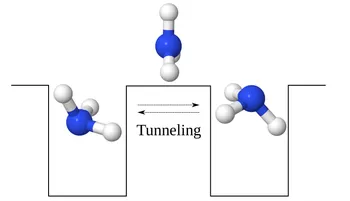
Another example is using the DSWP model to explain the ammonia maser. As shown in the figure above, the nitrogen in the NH molecule can oscillate up and down. Consider starting from an initial state, where the nitrogen is localized on the left quantum well. The wavefunction can be formulated as a combination of the two lowest quantum states.
The time-resolved state is written as (assuming real wavefunctions):
where the is defined as:
Therefore, the probability density is given as:
At , the wavefunction becomes localized in the right quantum well:
In this model, the nitrogen moves from left well to right well and back again with a frequency . As we already know, the energy difference is very small, which leads to a small frequency of the nitrogen inversion. The NH molecule emits radiation through this process.