Background Theory: Ising Model in 2D

Original notebook: theory_ising_model.ipynb

The Ising Model

Magnetism is an important physical property of materials. The Ising model is a simple and successful model to predict the net magnetization of a regular lattice of spins. Recently, it has been proven that it is actually a universal model beyond spin, and can also be applied to many other systems with similar model Hamiltonians (see e.g. De las Cuevas, Cubitt, Science 351, 1180 (2016)).

In this notebook, we construct a two-dimensional (2D) square Ising model and simulate its statistical properties at various temperatures with the Monte Carlo method (using a Metropolis-Hastings algorithm).

In the Ising model, spins can be in one of only two states: up (+) or down (-). In addition, the spin-spin interactions are considered to be non-zero only between nearest neighbours (NN), as illustrated in the figure below.

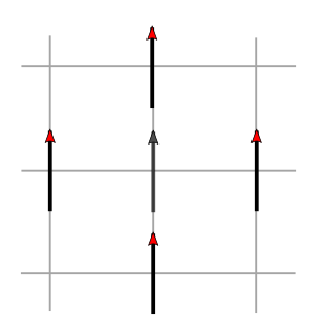
Nearest neighbours for a spin in a 2D lattice — In 2D, the gray spin has 4 nearest neighbours

In this approximation, the Hamiltonian of the Ising Model can be written as:

\large H = - \sum_{\langle i,j\rangle} J_{ij}\sigma_i \sigma_j - \sum_{i} h \sigma_i

where $J_{ij}$ the strength of spin-spin interaction (for simplicity we consider here a square model with a constant $J=J_{ij}$ ); $\langle i,j\rangle$ indicates summing on all nearest-neighbour pairs $(i, j)$ ; $h$ is an external field (we will consider no external field, $h=0$ , in the following); and $\sigma_i$ is the spin at site $i$ , that can take either the value $+1$ for a spin up, or $-1$ for a spin down.

Metropolis-Hastings

In this notebook, we simulate properties using the Monte Carlo method with a Metropolis-Hastings algorithm.

A description of the Metropolis-Hastings algorithm can be found in the notebook on Monte Carlo simulations to sample the canonical distribution.

Note that every “step”, here, represents a full sweep of all spins, with one actual Monte Carlo step per spin, where the move consists in flipping (accepted move) or not flipping (rejected move) the spin. Spins are traversed in a checkerboard pattern: first all spins with (even, even) coordinates are considered, then (even, odd), then (odd, even), and finally (odd, odd). When all spins have been considered, the “step” is considered as complete.

The Curie temperature

The Curie temperature ( $T_C$ ) is the temperature at which a material loses its permanent magnetic characteristics. The Curie temperature is named after the French physicist Pierre Curie.

In order to estimate $T_C$ from our simulations of the Ising model, we can perform simulations in a range of temperatures. For each simulation, we can run long enough to thermalize the simulation and obtain the stable spin configuration and the corresponding value of the magnetization per spin. We can then plot the magnetization per spin as a function of temperature $T$ . We expect that the magnetization per spin starts at 1 for $T=0$ and decreases for increasing $T$ . At $T_C$ , the magnetization will drop to zero and remain zero at higher temperatures.

Note that for a finite-size system, fluctuations will be present: therefore simulations for the same parameters will not give all the same result; rather, results will be distributed around the expected value. The magnitude of the fluctuations depends on the system size (larger fluctuations for smaller systems) and on how close are to the Curie temperature. We note, in particular, that one can obtain the magnetic susceptibility from the fluctuations of the magnetization. The magnetic susceptibility will diverge for $T=T_c$ (i.e., fluctuations will be very large close to the Curie temperature).