Background Theory: Monte Carlo calculation of Pi

Original notebook: theory_monte_carlo_pi.ipynb

Introduction

In mathematics, Monte Carlo integration is a method used to carry out numerical integration through use of random numbers. This method is particularly useful for high-dimensional integration.

Monte Carlo integration

The idea behind Monte Carlo integration is to evaluate the integral using random sampling. Basically, it can be done by sampling N points independently from the integration range and using these to approximate the integral as a finite sum. For a multidimensional definite integral:

\large I = \int_\Omega f(x)dx

where $\Omega$ has multidimensional volume:

\large V = \int_\Omega dx

Then sampling N points uniformly on $\Omega$ :

\large x_1, \cdot \cdot \cdot, x_N \in \Omega

$I$ can be approximated by:

\large I \approx Q_N\equiv V\frac{1}{N}\sum_{i=1}^{N}f(x_i) = V \langle f \rangle

A large number of samples is required in order to converge the value:

\large \lim_{N\to \infty} Q_N = I

Quasi-Monte Carlo integration

Unlike the regular Monte Carlo method using pseudorandom numbers, the quasi-Monte Carlo method uses so-called low-discrepancy sequences. Otherwise, Monte Carlo and quasi-Monte Carlo methods have identical underlying principles.

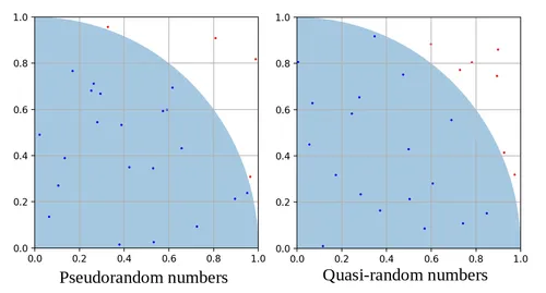
Low-discrepancy sequences are also called quasi-random numbers. The discrepancy of a sequence is a measure of its uniformity. Consider generating 25 random points on a 2D grid (5x5). Pseudorandom number generation typically leads to a cluster of points. To understand this, one may not that true randomness may not appear random on the surface. For instance, a coin may be flipped and land on tails for a surprisingly large number of consecutive flips. This is the nature of randomness. On the other hand, in the present example, low-discrepancy sequences fill each box with one point as shown in the figure below. This results in ostensibly greater randomness and better sampling. Using low-discrepancy sequences consequently leads to faster rates of convergence. Quasi-Monte Carlo has a convergence rate that goes like O(1/N). While the rate for the regular Monte Carlo method is O( $N^{-0.5}$ ).

Calculation of Pi

In the attached interactive notebook, we consider a simple Monte Carlo simulation to calculate the value of Pi. Suppose we have a square area which has sides of length 1 meter. We can throw coins into the square. The positions at which the coins fall are distributed randomly. We will have the follow relation:

\large \frac{\text{Area of a Quarter Circle}}{\text{Area of a Square}} \approx \frac{\text{Number of Coins inside the Circle}}{\text{Total Number of Coins}}

Hence, the value of Pi can be estimated as:

\large \pi \approx 4\times\frac{\text{Number of Coins inside the Circle}}{\text{Total Number of Coins}}