← Back to index

Numerical Solution of 1D Time Dependent Schrödinger Equation by Split Operator Fourier Transform (SOFT) Method

Authors: Dou Du, Taylor James Baird and Sara Bonella

Original notebook: soft.ipynb

This notebook presents the Split Operator Fourier Transform (SOFT) numerical method for solving the one-dimensional time-dependent Schrödinger equation.

Goals

• Use the SOFT method to observe the evolution of a quantum mechanical system in the coordinate ($X$) and momentum ($P$) representations using different potentials.
• Background theory: understand the steps involved in the SOFT algorithm and how they are translated to code.
• Explore how the performance of the simulations depends on different core parameters.
• As in the first point, observe the evolution of the system in the position and momentum representations and take note of the manifestation of Heisenberg’s uncertainty principle.

Background theory

More in the background theory.

Tasks and exercises

1. Investigate the dependence on timestep of the stability of the dynamics (move the slider for $dt$ and monitor the total energy of the system and norm of the wavefunction).

   Solution

   Observe that as the timestep employed in the simulation is increased, the conservation of total energy of the system degrades until eventually the timestep is so large that the dynamics becomes totally unstable. The reason why this integration scheme does not conserve total energy exactly may be attributed to the non-commutativity of the split-operator propagator with the Hamiltonian. It is worth noting, however, that norm conservation is maintained even as one increases the timestep. This latter fact is due to the unitarity of the propagator in the split-operator scheme.

2. What dictates the maximum size of the timestep that we can use for the SOFT algorithm (consider the main assumptions/approximations that are made when formulating the propagation scheme for SOFT).

   Solution

   Recall that the central approximation used in the derivation of the SOFT propagation scheme is in the truncation of the (symmetric) Trotter product formula: $e^{A+B} = \lim\limits_{P \to \infty} (e^{\frac{B}{2P}}e^{\frac{A}{P}} e^{\frac{B}{2P}})^{P} \approx (e^{\frac{B}{2N}}e^{\frac{A}{N}} e^{\frac{B}{2N}})^{N}$ for $N$ sufficiently large. This approximation becomes more and more accurate the larger we make the value of $N$. In our specific case we have $e^{\frac{it}{\hbar} (\hat{T} + \hat{V} )}$ and we approximate this via the product $(e^{\frac{it}{2\hbar N_{\text{steps}}}\hat{V} }e^{\frac{it}{\hbar N_{\text{steps}}}\hat{T} } e^{\frac{it}{2\hbar N_{\text{steps}}}\hat{V} })^{N_{\text{steps}}}$ where $N_{\text{steps}}\cdot dt = t$. This approximation therefore becomes increasingly more accurate the larger $N_{\text{steps}}$ (or equivalently the smaller we make $dt$).

3. Why is the use of the SOFT algorithm unfeasible for larger systems (think about how much data is needed to represent the state of the system on a computer and how many operations are required to carry out the propagation)?

   Solution

   In order to implement the SOFT algorithm on a computer it is necessary to discretize the nuclear wavefunction. To do so, we must introduce a grid of points that make up the space throughout which the wavefunction extends. Say that for each dimension of the grid we use $N$ grid points. For a system in $d$ dimensions, this means that we shall require $N^d$ points to represent the wavefunction of a single nucleus. Now, if we want to instead consider a system of, say $n$ nuclei, then we find that a total number of $N^{nd}$ grid points are required. In other words, the amount of data required to represent our system scales exponentially with increasing system size. Moreover, since we must loop over each of these grid points to carry out the time evolution of our system - the number of operations required also scales exponentially. This is what renders the SOFT algorithm unsuitable for large systems.

4. Observe the evolution of the wavefunction in both position and momentum space. Do you notice the manifestation of Heisenberg’s uncertainty principle? Can you explain it?

   Solution

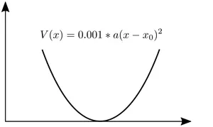
   The top figure shows the relation between position $x$ and the modulus of the wavefunction $|\psi|$. On the other hand, the bottom figure shows the relation between momentum $p$ and the modulus of the wavefunction, $|\psi|$. Using the Harmonic potential for example, one can clearly see that when the position of the particle is known with greater certainty (a sharp peak of the $|\psi(x)|$), the $|\psi(p)|$ will have a boarder shape. The phenomenon is always true during all the time.

Interactive visualization

Legend

(How to use the interactive visualization)

Interactive figures

The interactive figures consist of four subplots. Clockwise from the top left we have:

1. The evolution of the wavefunction in the position representation, $x$. The chosen potential is also shown in this subplot.
2. The evolution of the wavefunction in the momentum representation, $p$. The initial momentum $p_0$ (along with $-p_0$) are indicated with veritcal lines in this subplot.
3. Plot of the kinetic, potential and total energies vs simulation timestep (zoom to better discern the evolution of each contribution).
4. Evolution of the total norm of the nuclear wavepacket.

Controls

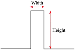
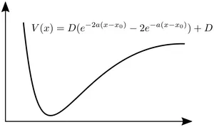
Before running the simulations, users need to select a potential and set various simulation parameters. We offer three types of potentials, namely the box, Morse and Harmonic potentials. One can also tune the parameters of these potentials. Moreover, the nuclear mass, $m$, and the size of the time step, $\Delta t$ may be modified via their corresponding sliders. Afterwards, one can click the “Play” button to run the simulation. One can also pause the simulation and reselect potential and reset parameters.

By default, the figures only show the absolute value of the wavefunction, $|\psi(x)|$. However, one can also select to show the real Re$(\psi(x))$ and image Im$(\psi(x))$ parts of the wavefunction by ticking the corresponding checkboxes.