← Go back to the interactive notebook
Background Theory: Numerical Solution of 1D Time Dependent Schrödinger Equation by Split Operator Fourier Transform (SOFT) Method Original notebook: theory_soft.ipynb
In other notebooks, we focus on numerical solutions of the time-independent Schrödinger equation. Here, we demonstrate the numerical solution of the one-dimensional time dependent Schrödinger equation. The split operator Fourier transform (SOFT) was employed.
Let’s consider a time-independent Hamiltonian and its associated time-dependent Schrödinger equation for a system of one particle in one dimension.
i ℏ d d t ∣ ψ ⟩ = H ^ ∣ ψ ⟩ where H ^ = P ^ 2 2 m + V ( X ^ ) \large i\hbar\frac{d}{dt}|\psi\rangle = \hat{H}|\psi\rangle \quad \text{where} \quad
\hat{H} = \frac{\hat{P}^2}{2m} + V(\hat{X}) i ℏ d t d ∣ ψ ⟩ = H ^ ∣ ψ ⟩ where H ^ = 2 m P ^ 2 + V ( X ^ ) We know that this equation admits at least a formal solution of the kind ∣ ψ ( t ) ⟩ = exp [ − i ℏ H ^ t ] ∣ ψ ( 0 ) ⟩ |\psi(t)\rangle = \exp\biggl[-\frac{i}{\hbar}\hat{H}t\biggr]|\psi(0)\rangle ∣ ψ ( t )⟩ = exp [ − ℏ i H ^ t ] ∣ ψ ( 0 )⟩ ψ ( X t , t ) = ∫ d X 0 K ( X t , t ; X 0 , 0 ) ψ ( X 0 , 0 ) \psi(X_t,t) = \int dX_0 K(X_t, t; X_0, 0)\psi(X_0,0) ψ ( X t , t ) = ∫ d X 0 K ( X t , t ; X 0 , 0 ) ψ ( X 0 , 0 ) K ( X t , t ; X 0 , 0 ) = ⟨ X t ∣ exp [ − i ℏ H ^ t ] ∣ X 0 ⟩ K(X_t, t; X_0, 0)= \langle X_t|\exp\biggl[-\frac{i}{\hbar}\hat{H}t\biggr]|X_0 \rangle K ( X t , t ; X 0 , 0 ) = ⟨ X t ∣ exp [ − ℏ i H ^ t ] ∣ X 0 ⟩ X t X_t X t X 0 X_0 X 0 X X X X ′ X' X ′
k ( X t , X 0 ) = ⟨ X t ∣ e − i ℏ H ^ t ∣ X 0 ⟩ = ⟨ X N + 1 ∣ e − i H ^ ℏ t / N e − i H ^ ℏ t / N . . . e − i H ^ ℏ t / N ⏟ N ∣ X 0 ⟩ \large k(X_t, X_0) = \langle X_t|e^{-\frac{i}{\hbar}\hat{H}t} | X_0 \rangle = \langle X_{N+1} | \underbrace{e^{-\frac{i\hat{H}}{\hbar}t/N} e^{-\frac{i\hat{H}}{\hbar}t/N} ... e^{-\frac{i\hat{H}}{\hbar}t/N}}_\textrm{N} |X_0 \rangle k ( X t , X 0 ) = ⟨ X t ∣ e − ℏ i H ^ t ∣ X 0 ⟩ = ⟨ X N + 1 ∣ N e − ℏ i H ^ t / N e − ℏ i H ^ t / N ... e − ℏ i H ^ t / N ∣ X 0 ⟩ Let us then focus on the single step propogator.
⟨ X 1 ∣ ψ ( ϵ ) ⟩ = ψ ( X 1 , ϵ ) = ∫ d X 0 ⟨ X 1 ∣ e − i ℏ H ^ ϵ ∣ X 0 ⟩ ψ ( X 0 , 0 ) \large \langle X_1 |\psi(\epsilon) \rangle = \psi(X_1,\epsilon) = \int dX_0 \langle X_1 |
e^{-\frac{i}{\hbar}\hat{H}\epsilon} |X_0 \rangle \psi(X_0,0) ⟨ X 1 ∣ ψ ( ϵ )⟩ = ψ ( X 1 , ϵ ) = ∫ d X 0 ⟨ X 1 ∣ e − ℏ i H ^ ϵ ∣ X 0 ⟩ ψ ( X 0 , 0 ) We can use the Trotter approximation to write:
⟨ X 1 ∣ e − i ℏ H ^ ϵ ∣ X 0 ⟩ = ⟨ X 1 ∣ e − i ℏ [ P 2 ^ 2 m + V ( X ^ ) ] ϵ ∣ X 0 ⟩ ≈ ⟨ X 1 ∣ e − i ℏ V ( X ^ ) ϵ / 2 e − i ℏ P 2 ^ 2 m ϵ e − i ℏ V ( X ^ ) ϵ / 2 ∣ X 0 ⟩ \large \langle X_1 |e^{-\frac{i}{\hbar}\hat{H}\epsilon}| X_0 \rangle = \langle X_1 | e^{-\frac{i}{\hbar}
[\frac{\hat{P^2}}{2m}+V(\hat{X})]\epsilon} | X_0\rangle \approx \langle X_1 | e^{-\frac{i}
{\hbar}V(\hat{X})\epsilon/2}e^{-\frac{i}{\hbar}\frac{\hat{P^2}}{2m}\epsilon}e^{-\frac{i}
{\hbar}V(\hat{X})\epsilon/2} | X_0 \rangle ⟨ X 1 ∣ e − ℏ i H ^ ϵ ∣ X 0 ⟩ = ⟨ X 1 ∣ e − ℏ i [ 2 m P 2 ^ + V ( X ^ )] ϵ ∣ X 0 ⟩ ≈ ⟨ X 1 ∣ e − ℏ i V ( X ^ ) ϵ /2 e − ℏ i 2 m P 2 ^ ϵ e − ℏ i V ( X ^ ) ϵ /2 ∣ X 0 ⟩ = e − i ℏ V ( X ^ ) ϵ / 2 ∫ d p ⟨ X 1 ∣ e − i ℏ P 2 ^ 2 m ϵ ∣ P ⟩ ⟨ P ∣ X 0 ⟩ e i ℏ V ( X ^ ) ϵ / 2 \large =e^{-\frac{i}{\hbar}V(\hat{X})\epsilon /2} \int dp \langle X_1 | e^{-\frac{i}{\hbar}\frac{\hat{P^2}}{2m}\epsilon} | P \rangle \langle P | X_0 \rangle e^{
\frac{i}{\hbar}V(\hat{X})\epsilon/2} = e − ℏ i V ( X ^ ) ϵ /2 ∫ d p ⟨ X 1 ∣ e − ℏ i 2 m P 2 ^ ϵ ∣ P ⟩ ⟨ P ∣ X 0 ⟩ e ℏ i V ( X ^ ) ϵ /2 where, ⟨ p ∣ X 0 ⟩ = 1 2 π ℏ e − i ℏ P X 0 \langle p | X_0 \rangle = \frac{1}{\sqrt{2\pi\hbar}}e^{-\frac{i}{\hbar}PX_0} ⟨ p ∣ X 0 ⟩ = 2 π ℏ 1 e − ℏ i P X 0
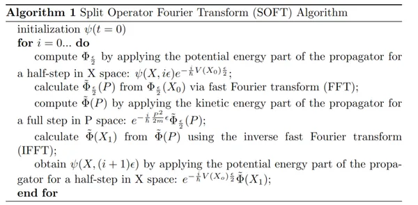
ψ ( X 1 , ϵ ) = e − 1 ℏ V ( X 1 ) ϵ / 2 ∫ d P 2 π ℏ e i ℏ P X 1 e − i ℏ P 2 2 m ϵ ∫ d X 0 2 π ℏ e − i ℏ P X 0 e − i ℏ V ( X 0 ) ϵ 2 ψ ( X 0 , 0 ) ⏟ Φ ϵ 2 ( X 0 ) ⏟ Φ ~ ϵ 2 ( P ) \large \psi(X_1,\epsilon)=e^{-\frac{1}{\hbar}V(X_1)\epsilon/2}\int \frac{dP}{\sqrt{2\pi\hbar}}e^{\frac{i}{\hbar}PX_1}e^{-\frac{i}{\hbar}\frac{P^2}{2m}\epsilon}\underbrace{\int \frac{dX_0}{\sqrt{2\pi\hbar}}e^{-\frac{i}{\hbar}PX_0}\underbrace{e^{-\frac{i}{\hbar}V(X_0)\frac{\epsilon}{2}}\psi(X_0,0)}_{\Phi_{\frac{\epsilon}{2}}(X_0)}}_{\tilde{\Phi}_{\frac{\epsilon}{2}}(P)} ψ ( X 1 , ϵ ) = e − ℏ 1 V ( X 1 ) ϵ /2 ∫ 2 π ℏ d P e ℏ i P X 1 e − ℏ i 2 m P 2 ϵ Φ ~ 2 ϵ ( P ) ∫ 2 π ℏ d X 0 e − ℏ i P X 0 Φ 2 ϵ ( X 0 ) e − ℏ i V ( X 0 ) 2 ϵ ψ ( X 0 , 0 ) ψ ( X 1 , ϵ ) = e − 1 ℏ V ( X 1 ) ϵ / 2 ∫ d P 2 π ℏ e i ℏ P X 1 e − i ℏ P 2 2 m ϵ Φ ~ ϵ 2 ( P ) ⏟ Φ ~ ( P ) ⏟ Φ ~ ( X 1 ) , \large \psi(X_1,\epsilon)=e^{-\frac{1}{\hbar}V(X_1)\epsilon/2}\underbrace{\int \frac{dP}{\sqrt{2\pi\hbar}}e^{\frac{i}{\hbar}PX_1}\underbrace{e^{-\frac{i}{\hbar}\frac{P^2}{2m}\epsilon}\tilde{\Phi}_{\frac{\epsilon}{2}}(P)}_{\tilde{\Phi}(P)}}_{\tilde{\Phi}(X_1)}, ψ ( X 1 , ϵ ) = e − ℏ 1 V ( X 1 ) ϵ /2 Φ ~ ( X 1 ) ∫ 2 π ℏ d P e ℏ i P X 1 Φ ~ ( P ) e − ℏ i 2 m P 2 ϵ Φ ~ 2 ϵ ( P ) , where we recognize Φ ~ ( P ) \tilde{\Phi}(P) Φ ~ ( P ) Φ ( X ) \Phi(X) Φ ( X )
By interating N times, we can obtain ψ ( X , t ) \psi(X,t) ψ ( X , t )